The Multiplication Rule of Probabilities

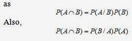
Let A and B be two events. Using the multiplication rule of probabilities, the probability of their intersection can be derived from conditional probability

Example: Product Choice: Ketchup and Mustard-When the conditional probability of mustard usage, given ketchup usage,is multiplied by the probability of ketchup usage, then we have the joint probability of both mustard and ketchup usage:

Example: Sensitive Questions (Multiplication Rule)
Suppose that a survey was carried out in New York, and each respondent was faced with the following two questions:
a.    Is the last digit of your Social Security number odd?
b.    Have you ever lied on an employment application?

The second question is, of course, quite sensitive, and for various reasons we might expect that a number of people would not answer the question honestly, especially if their response was yes. To overcome this potential bias, respondents were asked to flip a coin and then to answer question (a) if the result was “head” and (b) otherwise. A “yes” response was given by 37%of all respondents. What is the probability that a respondent who was answering the sensitive question, (b), replied “yes”?                   

Solution: We define the following events:
       A: Respondent answers “yes.”
       E1: Respondent answers question (a).
       E2: Respondent answers question (b).

From the problem discussion we know that P(A) = 0.37. We know that the choice if question was determined by a flip of a coin and that P(E1) = 0.5 and P(E2) = 0.5. In addition, we know the answers to question (a). Since half of all Social Security numbers have an odd last digit, it must be that the probability of a “yes” answer, given that question (a) has been answered, is 0.5—that is, P(A/E1) = 0.50.

However, we require P(A/E2), the conditional probability of a “yes” response, given that question (b) was answered. We can obtain this probability by using two results from previous sections. We know that E1 and E2 are mutually exclusive and collectively exhaustive.

From the result, we estimate that 24% of the surveyed population has lied on some employment application.

Statistical Independence

Let A and B be two events. These events are said to be statistically independent if and only if

The logical basis for the definition of statistical independence is best seen in terms conditional probabilities and is most appealing from a subjective view of probability. Suppose that I believe the probability that event A will occur is P(A). Then I am given the information that event B has occurred. If this new information does not change my view of the probability of A,
 then P(A) = P(A/B), and the information about the occurrence of B is of no value in determining P(A). This definition of statistical independence agrees with a commonsense notion of “independence”.

Example: Probability of College Degrees (Statistical Independence)
Suppose that women obtain 48% of all bachelor degrees in a particular country and that 17.5% of all bachelor degrees are in business. Also, 6% of all bachelor degrees go to women majoring in business. Are the events “Bachelor degree holder is a women” and “Bachelor degree is in business” statistically independent? 

Solution: Let A denote the vent “Bachelor degree holder is a women” and B the event “Bachelor degree is in business” and we have

Thus, in the country of interest only 34.3% of business degrees go to women, whereas women const itute 48% of all degree recipients.

Scatter Plot (or Scatter Diagram)

 Business and economic analyses are often concerned about relationships between variables. Do higher SAT mathematics scores predict higher collage GPAs? What is the change in quantity sold as the result of a change in price? How are total sales influenced by total disposable income in a geographic region? Does advertising increase sales? What is the change in infant mortality in developing countries as per capita income increases?

In these examples we notice that one variable may depend to a certain extent on the other variable. For example, a student’s GPA may depend on his or her SAT math score, We then call GPA the dependent variable and label it Y. We call SAT math score the independent variable and label it X. Similarly, we would label the quantity sold as Y and the price of a commodity as X.

To answer these questions, we gather and analyze random samples of data collected from relevant populations.

A scatter diagram insight as the to the relationship that may exist between two variables. We can prepare a scatter plot by locating one point for each pair of two variables that represent an observation in the data set. The scatter plot provides a picture of the data, including the following:

1.    The range of each variable.
2.    The pattern of values over the range
3.    A suggestion as to a possible relationship between the two variables
4.    An indication of outliers (extreme points)

We could prepare scatter plots by plotting individual points on graph paper. However, all modern statistical packages contain routines for preparing scatter plots directly from an electronic data file.

Example: Table below gives the SAT math scores from a test given before admission to college and the GPAs at college graduation for a random sample of 11 students at one small private university. Draw a scatter plot and determine what information it provides.

SAT MATH	450	480	500	520	560	580	590	600	620	650	700
GPA	3.25	2.60	2.88	2.85	3.30	3.10	3.35	3.20	3.50	3.59	3.95

Solution: Using Excel, we obtain the flowing Figure, a scatter plot of the dependent variable, college GPA, and the independent variable, SAT math score. An interesting pattern is the positive upward trend—GPA scores tend to increase directly with increases in SAT math scores. Note also that the relationship does not provide an exact prediction. Some students with low SAT math scores have higher GPA scores than do students with higher SAT math scores. We that the basic pattern indicates that higher entrance scores predict higher grade point averages, but the results are not perfect.

Covariance

Covariance (Cov) is a measure of the linear relationship between two variables. A positive value indicates a direct or increasing linear relationship, and a negative value indicates a decreasing linear relationship.

The sample correlation coefficient will give us a standardized measure of the linear relationship between two variables. It is generally a more useful measure, as it provides both the direction and the strength of relationship. The covariance and corresponding correlation coefficient have same sign (both are positive o both are negative).

Correlation Coefficient

The correlation coefficient is computed by dividing the covariance by the product of the standard deviations of the two variables.

The correlation coefficient ranges from –1 to +1. The closer r is  to +1, the closer the data points are to an increasing straight line indicating a positive linear relationship. The closer r is to –1, the closer the data points are to a decreasing straight line indicating a negative linear relationship. When r = 0, there is no linear relationship between x and y but not necessarily a lack of relationship. 

Example: Rising Hills Manufacturing Inc. wishes to study the relationship between the number of workers, X, and the number of tables, Y, produced in its Redwood Falls plant. It has obtained a random samples of 10 hours of production. The following (x, y) combinations of points were obtained:
       (12, 20)             (30, 60)     (15, 27)        (24, 50)   (14, 21)
       (18, 30)             (28, 61)     (26, 54)        (19, 32)   (27, 57)

Compute the covariance and correlation coefficient. Discuss briefly the relationship between the number of workers and the number of tables produced per hour.

Solution: The computations are set out in the Table bellow.

We conclude that there is a strong positive relationship between number of workers and number of tables produced per hour.

Obtaining Linear Relationships

We have now seen how the relationship between two variables can be described by using sample data. Scatter plots provide a picture of the relationship, and correlation coefficients provide a numerical measure. In many economic and business problems a specific functional relationship is desired.

•    What mean level of sales can be expressed if the price is set at $10 per unit?
•    If 250 workers are employed, how many units should be expected?
•    If a developing country increases its fertilizer production by 1,000,000 tons, how much increase in grain production should be expected?

Economic models use specific functional relationship to indicate the effect on a dependent variable, Y, that results from various changes in an independent or input variable, X. In many cases we can adequately approximate the desired functional relationships by a linear equation:

 where Y is the dependent variable, X is the independent variable, is the Y-intercept, and is the slope of the line, or the change in Y for every unit change in X. The linear equation model computes the mean of Y for every value of X. This idea is the basis for obtaining many economic and business relationships, including demand functions, production functions, consumption functions, and sales forecasts.

We use regression to determine the best relationship between Y and X for a particular application. This requires us to the best values for the coefficients  and . Generally, we use the data available from the process to compute “estimates” or numerical values for the coefficients  and These estimates—defined as  b0 and b1 --are generally computed by the leas squares regression. Least-squares is a procedure that selects the best-fit line, given a set of data points.

The linear equation represented by the line is the best-fit linear equation. We see that individual data points are above and below the line and that the line has points with both positive and negative deviations. The distance of each point (xi, yi) from the linear equation is defined as residual, ei. We would like to choose the equation so that some function of the positive and negative residuals is as small as possible. This implies finding estimates for the coefficients and . 

Least-squares regression chooses b0 and b1 such that the sum of the squared residuals is minimized.

Least-Squares Regression

The lest-squares regression line based on sample data is

b1 is the slope of the line, or the change in y for every unit change in x, and is calculated as

where b0 is the y-intercept and is calculated as

Example: Rising Hills Manufacturing Inc. wishes to study the relationship between the number of workers, X, and the number of tables, Y, produced in its Redwood Falls plant. It has obtained a random samples of 10 hours of production. The following (x, y) combinations of points were obtained:
       (12, 20)             (30, 60)     (15, 27)        (24, 50)   (14, 21)
       (18, 30)             (28, 61)     (26, 54)        (19, 32)   (27, 57)

Compute the covariance and correlation coefficient. Discuss briefly the relationship between the number of workers and the number of tables produced per hour.

Solution: The computations are set out in the Table bellow.

From the covariance we see that the direction of the relationship is positive, the high correlation of 0.989 also indicate that the same data points are very close to some increasing straight line.

We can also use a statistical software package such as Minitab or spreadsheet such as Excel to obtain the same regression coefficients and regression line.